How DLW works

A quick summary of how the DLW method�works

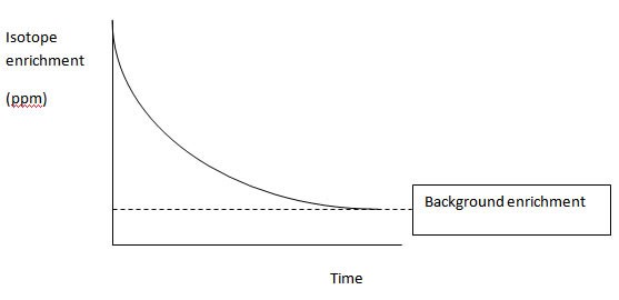
Isotopes introduced into the body get washed out by the flux of materials that carry the elements of those isotopes.� The elimination pattern follows an exponential decline as the enrichment of the specific isotope gets more and more depleted and returns to the background enrichment level� (see Fig 1).�

�

Figure 1: isotope elimination

�

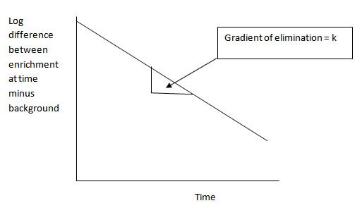
To characterise this elimination pattern a semi-log plot is generated (Fig 2) of the logged difference between the enrichment and the background enrichment over time. This process linearises the relationship. The gradient of this line (normally represented by k) represents the isotope washout rate. To get the actual rate at which this element is being flushed through the body you simply multiply this gradient by the size of the pool that is being turned over (normally represented by N)�

Figure 2: isotope elimination on semi-log plot to linearise the curve.

�

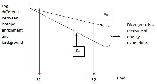
The body water is made up of hydrogen and oxygen. If you introduce an isotope of hydrogen (deuterium or tritium) into the body it will be washed out by the constant inflow of water (preformed in our food, what we drink and metabolic water formed when we metabolise food) and the constant outflow (as urine, sweat, evaporation from our mouths). If you introduce an isotope of oxygen (oxygen-17 or oxygen-18) it is also washed out by all these same routes. However, isotopic oxygen is also flushed out of the system�by�the constant intake of oxygen and the constant removal of carbon dioxide. So over time the isotope enrichments for hydrogen (kH) and oxygen (ko) diverge (Fig 3).

Figure 3: divergence of labels of oxygen and hydrogen over time.

�

The difference between the washout curves is then a reflection of the rate at which oxygen and CO2 pass through the body, which is a measure of energy expenditure.�The real benefit of the method is that because the log converted�elimination lines are linear, one only needs to collect samples at two time points to characterise the two elimination curves (S1 and S2 in Fig 3). Between these time points the subject can go about their daily routines as normal. The technique therefore provides an estimate of free-living energy demands. This has been variously called DEE (daily energy expenditure), TEE (Total energy expenditure) or FMR (Field metabolic rate).